This Jupyter notebook can be downloaded from rednoise-fit-example.ipynb, or viewed as a python script at rednoise-fit-example.py.
Red noise, DM noise, and chromatic noise fitting examples
This notebook provides an example on how to fit for red noise and DM noise using PINT using simulated datasets.
We will use the PLRedNoise and PLDMNoise models to generate noise realizations (these models provide Fourier Gaussian process descriptions of achromatic red noise and DM noise respectively).
We will fit the generated datasets using the WaveX and DMWaveX models, which provide deterministic Fourier representations of achromatic red noise and DM noise respectively.
Finally, we will convert the WaveX/DMWaveX amplitudes into spectral parameters and compare them with the injected values.
[1]:
from pint import DMconst
from pint.models import get_model
from pint.simulation import make_fake_toas_uniform
from pint.logging import setup as setup_log
from pint.fitter import WLSFitter
from pint.utils import (
    cmwavex_setup,
    dmwavex_setup,
    find_optimal_nharms,
    plchromnoise_from_cmwavex,
    wavex_setup,
    plrednoise_from_wavex,
    pldmnoise_from_dmwavex,
)

from io import StringIO
import numpy as np
import astropy.units as u
from matplotlib import pyplot as plt
from copy import deepcopy

setup_log(level="WARNING")
[1]:
1
Red noise fitting
Simulation
The first step is to generate a simulated dataset for demonstration. Note that we are adding PHOFF as a free parameter. This is required for the fit to work properly.
[2]:
par_sim = """
    PSR           SIM3
    RAJ           05:00:00     1
    DECJ          15:00:00     1
    PEPOCH        55000
    F0            100          1
    F1            -1e-15       1
    PHOFF         0            1
    DM            15           1
    TNREDAMP      -13
    TNREDGAM      3.5
    TNREDC        30
    TZRMJD        55000
    TZRFRQ        1400
    TZRSITE       gbt
    UNITS         TDB
    EPHEM         DE440
    CLOCK         TT(BIPM2019)
"""

m = get_model(StringIO(par_sim))
[3]:
# Now generate the simulated TOAs.
ntoas = 2000
toaerrs = np.random.uniform(0.5, 2.0, ntoas) * u.us
freqs = np.linspace(500, 1500, 8) * u.MHz

t = make_fake_toas_uniform(
    startMJD=53001,
    endMJD=57001,
    ntoas=ntoas,
    model=m,
    freq=freqs,
    obs="gbt",
    error=toaerrs,
    add_noise=True,
    add_correlated_noise=True,
    name="fake",
    include_bipm=True,
    multi_freqs_in_epoch=True,
)
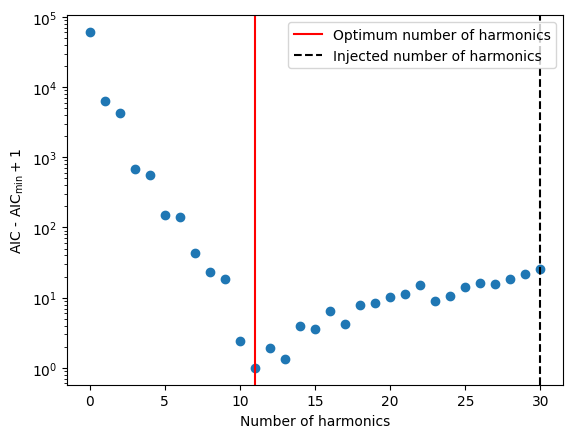
Optimal number of harmonics
The optimal number of harmonics can be estimated by minimizing the Akaike Information Criterion (AIC). This is implemented in the pint.utils.find_optimal_nharms function.
[4]:
m1 = deepcopy(m)
m1.remove_component("PLRedNoise")

nharm_opt, d_aics = find_optimal_nharms(m1, t, "WaveX", 30)

print("Optimum no of harmonics = ", nharm_opt)
Optimum no of harmonics = 11
[5]:
print(np.argmin(d_aics))
11
[6]:
# The Y axis is plotted in log scale only for better visibility.
plt.scatter(list(range(len(d_aics))), d_aics + 1)
plt.axvline(nharm_opt, color="red", label="Optimum number of harmonics")
plt.axvline(
    int(m.TNREDC.value), color="black", ls="--", label="Injected number of harmonics"
)
plt.xlabel("Number of harmonics")
plt.ylabel("AIC - AIC$_\\min{} + 1$")
plt.legend()
plt.yscale("log")
# plt.savefig("sim3-aic.pdf")
[7]:
# Now create a new model with the optimum number of harmonics
m2 = deepcopy(m1)
Tspan = t.get_mjds().max() - t.get_mjds().min()
wavex_setup(m2, T_span=Tspan, n_freqs=nharm_opt, freeze_params=False)

ftr = WLSFitter(t, m2)
ftr.fit_toas(maxiter=10)
m2 = ftr.model

print(m2)
# Created: 2026-05-01T15:04:15.891413
# PINT_version: 1.1.4+112.g3f5c736
# User: docs
# Host: build-32499821-project-85767-nanograv-pint
# OS: Linux-7.0.0-1004-aws-x86_64-with-glibc2.35
# Python: 3.11.14 (main, Apr 27 2026, 17:28:30) [GCC 11.4.0]
# Format: pint
# read_time: 2026-05-01T15:03:28.977653
# allow_tcb: False
# convert_tcb: False
# allow_T2: False
PSR                                  SIM3
EPHEM                               DE440
CLOCK                        TT(BIPM2019)
UNITS                                 TDB
START              53000.9999999566028241
FINISH             56985.0000000463068981
DILATEFREQ                              N
DMDATA                                  N
NTOA                                 2000
CHI2                   2020.7178892989039
CHI2R                  1.0252247028406412
TRES                0.9994003611563433042
RAJ                      4:59:59.99998453 1 0.00001808261118507026
DECJ                    15:00:00.00411271 1 0.00191771162093936883
PMRA                                  0.0
PMDEC                                 0.0
PX                                    0.0
F0                 100.000000000000088866 1 1.626848095765143481e-13
F1              -1.0000486380320161993e-15 1 6.617444007680447296e-20
PEPOCH             55000.0000000000000000
PLANET_SHAPIRO                          N
DM                  14.999995817939726093 1 4.6750032179890137183e-06
WXEPOCH            55000.0000000000000000
WXFREQ_0001        0.00025100401605860576
WXSIN_0001         1.7979616869959129e-06 1 1.8324995181191947e-07
WXCOS_0001         1.0010602027147485e-05 1 3.983905191089185e-06
WXFREQ_0002         0.0005020080321172115
WXSIN_0002           9.48658606868778e-07 1 9.516253092667091e-08
WXCOS_0002        -1.8862316212933826e-06 1 1.0026202357560626e-06
WXFREQ_0003         0.0007530120481758173
WXSIN_0003         2.0188084411705946e-06 1 6.903785042850568e-08
WXCOS_0003         4.5758152658280184e-07 1 4.528932213473466e-07
WXFREQ_0004          0.001004016064234423
WXSIN_0004         3.1768026434249494e-07 1 5.629652604978996e-08
WXCOS_0004         -9.352403164602336e-07 1 2.612792786449312e-07
WXFREQ_0005         0.0012550200802930289
WXSIN_0005          5.438338542842225e-07 1 5.0232699823690013e-08
WXCOS_0005          1.000232816750356e-06 1 1.7457074358372469e-07
WXFREQ_0006         0.0015060240963516347
WXSIN_0006          9.325558367342482e-08 1 4.714099521109552e-08
WXCOS_0006          -3.87859791446348e-07 1 1.289682093068257e-07
WXFREQ_0007         0.0017570281124102405
WXSIN_0007         -6.894667578616771e-09 1 4.5021101014087236e-08
WXCOS_0007          5.020001865389287e-07 1 1.0279022485576901e-07
WXFREQ_0008          0.002008032128468846
WXSIN_0008          -8.68661273826864e-08 1 4.508944516526302e-08
WXCOS_0008          7.288257501916563e-09 1 8.882787324217385e-08
WXFREQ_0009          0.002259036144527452
WXSIN_0009         -8.683753781337331e-08 1 4.8113539470993794e-08
WXCOS_0009         1.1644352735073252e-07 1 8.631498328683403e-08
WXFREQ_0010         0.0025100401605860577
WXSIN_0010         1.1428156390273715e-07 1 6.60104273425186e-08
WXCOS_0010        -2.1652313543826123e-07 1 1.0711725555690236e-07
WXFREQ_0011         0.0027610441766446636
WXSIN_0011         -2.988525148202316e-07 1 4.2346435506330224e-07
WXCOS_0011         -1.256150088451366e-06 1 5.826128256760244e-07
TZRMJD             55000.0000000000000000
TZRSITE                               gbt
TZRFRQ                             1400.0
PHOFF               0.0006401549800269074 1 0.00032839324323180206
Estimating the spectral parameters from the WaveX fit.
[8]:
# Get the Fourier amplitudes and powers and their uncertainties.
idxs = np.array(m2.components["WaveX"].get_indices())
a = np.array([m2[f"WXSIN_{idx:04d}"].quantity.to_value("s") for idx in idxs])
da = np.array([m2[f"WXSIN_{idx:04d}"].uncertainty.to_value("s") for idx in idxs])
b = np.array([m2[f"WXCOS_{idx:04d}"].quantity.to_value("s") for idx in idxs])
db = np.array([m2[f"WXCOS_{idx:04d}"].uncertainty.to_value("s") for idx in idxs])
print(len(idxs))

P = (a**2 + b**2) / 2
dP = ((a * da) ** 2 + (b * db) ** 2) ** 0.5

f0 = (1 / Tspan).to_value(u.Hz)
fyr = (1 / u.year).to_value(u.Hz)
11
[9]:
# We can create a `PLRedNoise` model from the `WaveX` model.
# This will estimate the spectral parameters from the `WaveX`
# amplitudes.
m3 = plrednoise_from_wavex(m2)
print(m3)
# Created: 2026-05-01T15:04:15.934442
# PINT_version: 1.1.4+112.g3f5c736
# User: docs
# Host: build-32499821-project-85767-nanograv-pint
# OS: Linux-7.0.0-1004-aws-x86_64-with-glibc2.35
# Python: 3.11.14 (main, Apr 27 2026, 17:28:30) [GCC 11.4.0]
# Format: pint
# read_time: 2026-05-01T15:03:28.977653
# allow_tcb: False
# convert_tcb: False
# allow_T2: False
PSR                                  SIM3
EPHEM                               DE440
CLOCK                        TT(BIPM2019)
UNITS                                 TDB
START              53000.9999999566028241
FINISH             56985.0000000463068981
DILATEFREQ                              N
DMDATA                                  N
NTOA                                 2000
CHI2                   2020.7178892989039
CHI2R                  1.0252247028406412
TRES                0.9994003611563433042
RAJ                      4:59:59.99998453 1 0.00001808261118507026
DECJ                    15:00:00.00411271 1 0.00191771162093936883
PMRA                                  0.0
PMDEC                                 0.0
PX                                    0.0
F0                 100.000000000000088866 1 1.626848095765143481e-13
F1              -1.0000486380320161993e-15 1 6.617444007680447296e-20
PEPOCH             55000.0000000000000000
PLANET_SHAPIRO                          N
DM                  14.999995817939726093 1 4.6750032179890137183e-06
TZRMJD             55000.0000000000000000
TZRSITE                               gbt
TZRFRQ                             1400.0
PHOFF               0.0006401549800269074 1 0.00032839324323180206
TNREDAMP              -12.863157264177183 0 0.15355944536088384
TNREDGAM               3.4460467573699844 0 0.6711599996848779
TNREDC                                 11
[10]:
# Now let us plot the estimated spectrum with the injected
# spectrum.
plt.subplot(211)
plt.errorbar(
    idxs * f0,
    b * 1e6,
    db * 1e6,
    ls="",
    marker="o",
    label="$\\hat{a}_j$ (WXCOS)",
    color="red",
)
plt.errorbar(
    idxs * f0,
    a * 1e6,
    da * 1e6,
    ls="",
    marker="o",
    label="$\\hat{b}_j$ (WXSIN)",
    color="blue",
)
plt.axvline(fyr, color="black", ls="dotted")
plt.axhline(0, color="grey", ls="--")
plt.ylabel("Fourier coeffs ($\mu$s)")
plt.xscale("log")
plt.legend(fontsize=8)

plt.subplot(212)
plt.errorbar(
    idxs * f0, P, dP, ls="", marker="o", label="Spectral power (PINT)", color="k"
)
P_inj = m.components["PLRedNoise"].get_noise_weights(t)[::2][:nharm_opt]
plt.plot(idxs * f0, P_inj, label="Injected Spectrum", color="r")
P_est = m3.components["PLRedNoise"].get_noise_weights(t)[::2][:nharm_opt]
print(len(idxs), len(P_est))
plt.plot(idxs * f0, P_est, label="Estimated Spectrum", color="b")
plt.xscale("log")
plt.yscale("log")
plt.ylabel("Spectral power (s$^2$)")
plt.xlabel("Frequency (Hz)")
plt.axvline(fyr, color="black", ls="dotted", label="1 yr$^{-1}$")
plt.legend()
11 11
[10]:
<matplotlib.legend.Legend at 0x7854ee7bbd10>
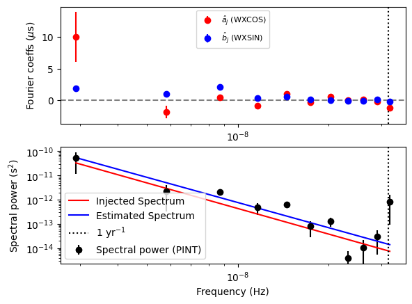
Note the outlier in the 1 year^-1 bin. This is caused by the covariance with RA and DEC, which introduce a delay with the same frequency.
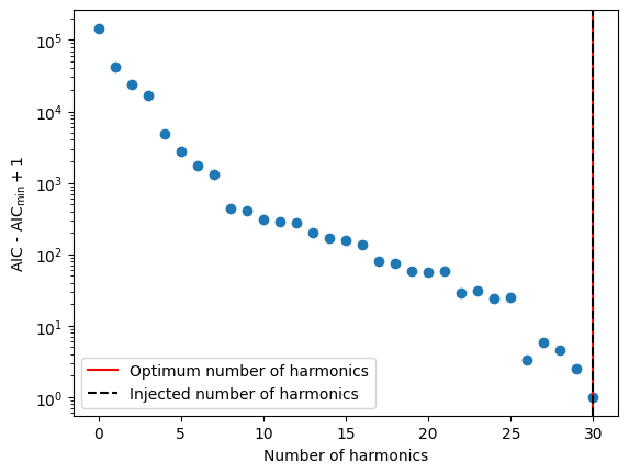
DM noise fitting
Let us now do a similar kind of analysis for DM noise.
[11]:
par_sim = """
    PSR           SIM4
    RAJ           05:00:00     1
    DECJ          15:00:00     1
    PEPOCH        55000
    F0            100          1
    F1            -1e-15       1
    PHOFF         0            1
    DM            15           1
    TNDMAMP       -13
    TNDMGAM       3.5
    TNDMC         30
    TZRMJD        55000
    TZRFRQ        1400
    TZRSITE       gbt
    UNITS         TDB
    EPHEM         DE440
    CLOCK         TT(BIPM2019)
"""

m = get_model(StringIO(par_sim))
[12]:
# Generate the simulated TOAs.
ntoas = 2000
toaerrs = np.random.uniform(0.5, 2.0, ntoas) * u.us
freqs = np.linspace(500, 1500, 8) * u.MHz

t = make_fake_toas_uniform(
    startMJD=53001,
    endMJD=57001,
    ntoas=ntoas,
    model=m,
    freq=freqs,
    obs="gbt",
    error=toaerrs,
    add_noise=True,
    add_correlated_noise=True,
    name="fake",
    include_bipm=True,
    multi_freqs_in_epoch=True,
)
[13]:
# Find the optimum number of harmonics by minimizing AIC.
m1 = deepcopy(m)
m1.remove_component("PLDMNoise")

m2 = deepcopy(m1)

nharm_opt, d_aics = find_optimal_nharms(m2, t, "DMWaveX", 30)
print("Optimum no of harmonics = ", nharm_opt)
Optimum no of harmonics = 30
[14]:
# The Y axis is plotted in log scale only for better visibility.
plt.scatter(list(range(len(d_aics))), d_aics + 1)
plt.axvline(nharm_opt, color="red", label="Optimum number of harmonics")
plt.axvline(
    int(m.TNDMC.value), color="black", ls="--", label="Injected number of harmonics"
)
plt.xlabel("Number of harmonics")
plt.ylabel("AIC - AIC$_\\min{} + 1$")
plt.legend()
plt.yscale("log")
# plt.savefig("sim3-aic.pdf")
[15]:
# Now create a new model with the optimum number of
# harmonics
m2 = deepcopy(m1)

Tspan = t.get_mjds().max() - t.get_mjds().min()
dmwavex_setup(m2, T_span=Tspan, n_freqs=nharm_opt, freeze_params=False)

ftr = WLSFitter(t, m2)
ftr.fit_toas(maxiter=10)
m2 = ftr.model

print(m2)
# Created: 2026-05-01T15:05:12.020809
# PINT_version: 1.1.4+112.g3f5c736
# User: docs
# Host: build-32499821-project-85767-nanograv-pint
# OS: Linux-7.0.0-1004-aws-x86_64-with-glibc2.35
# Python: 3.11.14 (main, Apr 27 2026, 17:28:30) [GCC 11.4.0]
# Format: pint
# read_time: 2026-05-01T15:04:16.567219
# allow_tcb: False
# convert_tcb: False
# allow_T2: False
PSR                                  SIM4
EPHEM                               DE440
CLOCK                        TT(BIPM2019)
UNITS                                 TDB
START              53000.9999999567105903
FINISH             56985.0000000465773148
DILATEFREQ                              N
DMDATA                                  N
NTOA                                 2000
CHI2                   1898.4189306027733
CHI2R                  0.9821101555110053
TRES               0.97321526471865212683
RAJ                      4:59:59.99999934 1 0.00000185847524176867
DECJ                    14:59:59.99976765 1 0.00016145911506297193
PMRA                                  0.0
PMDEC                                 0.0
PX                                    0.0
F0                  99.999999999999960205 1 3.5775429124952155762e-14
F1              -1.0000005446635623846e-15 1 8.169821965702234221e-22
PEPOCH             55000.0000000000000000
PLANET_SHAPIRO                          N
DM                  15.000007761618252591 1 4.967224699950917705e-06
DMWXEPOCH          55000.0000000000000000
DMWXFREQ_0001      0.00025100401605859476
DMWXSIN_0001       -0.0013533329149485974 1 5.994488881418064e-06
DMWXCOS_0001       -0.0002726923345966824 1 6.800251464527488e-06
DMWXFREQ_0002       0.0005020080321171895
DMWXSIN_0002      -2.1165494117996558e-05 1 4.805638138415625e-06
DMWXCOS_0002        0.0005774995140370753 1 4.496944896366989e-06
DMWXFREQ_0003       0.0007530120481757844
DMWXSIN_0003       -0.0003687587780133837 1 4.575569230627277e-06
DMWXCOS_0003      -0.00010428141219340168 1 4.296765716205425e-06
DMWXFREQ_0004        0.001004016064234379
DMWXSIN_0004       0.00037243881708276733 1 4.423170507601408e-06
DMWXCOS_0004      -0.00027426266413091595 1 4.342472298315879e-06
DMWXFREQ_0005        0.001255020080292974
DMWXSIN_0005       0.00012925900795716168 1 4.356563314845659e-06
DMWXCOS_0005       0.00016208131882494643 1 4.352390575300141e-06
DMWXFREQ_0006       0.0015060240963515688
DMWXSIN_0006       -9.230553455520815e-05 1 4.391703354896001e-06
DMWXCOS_0006        9.986320155170327e-05 1 4.282707641677931e-06
DMWXFREQ_0007       0.0017570281124101635
DMWXSIN_0007        1.659908622222018e-05 1 4.387253354571338e-06
DMWXCOS_0007        8.448147656692251e-05 1 4.272912809899521e-06
DMWXFREQ_0008        0.002008032128468758
DMWXSIN_0008       -0.0001228877691699294 1 4.383961016295776e-06
DMWXCOS_0008       5.8193018658339397e-05 1 4.254525101961086e-06
DMWXFREQ_0009        0.002259036144527353
DMWXSIN_0009       -2.298899997866944e-05 1 4.376543588065091e-06
DMWXCOS_0009        6.232770998953232e-06 1 4.2712309961788045e-06
DMWXFREQ_0010        0.002510040160585948
DMWXSIN_0010      -2.9734590477405463e-05 1 4.304555696221749e-06
DMWXCOS_0010       -2.804154633674839e-05 1 4.38995624473846e-06
DMWXFREQ_0011       0.0027610441766445426
DMWXSIN_0011      -1.0465057682152319e-05 1 6.8481380774684605e-06
DMWXCOS_0011        3.622317632218167e-05 1 7.0662957603507575e-06
DMWXFREQ_0012       0.0030120481927031375
DMWXSIN_0012        7.826363502377315e-06 1 4.335190908360838e-06
DMWXCOS_0012        1.076471981619795e-05 1 4.357208605000105e-06
DMWXFREQ_0013        0.003263052208761732
DMWXSIN_0013        3.204075845158531e-05 1 4.3936112763211055e-06
DMWXCOS_0013       -4.756285438781995e-06 1 4.257674250748948e-06
DMWXFREQ_0014        0.003514056224820327
DMWXSIN_0014       1.8009028576852022e-05 1 4.3018971505078745e-06
DMWXCOS_0014        1.785129352227688e-05 1 4.336401186281373e-06
DMWXFREQ_0015       0.0037650602408789216
DMWXSIN_0015        1.543328281124352e-05 1 4.307047253601188e-06
DMWXCOS_0015       1.2577778418117968e-05 1 4.329166682095992e-06
DMWXFREQ_0016        0.004016064256937516
DMWXSIN_0016        8.211721663763466e-06 1 4.291394955848233e-06
DMWXCOS_0016      -1.9021697861827038e-05 1 4.343890350457181e-06
DMWXFREQ_0017       0.0042670682729961116
DMWXSIN_0017        3.918038495957322e-07 1 4.36994645645138e-06
DMWXCOS_0017       -3.192632459616425e-05 1 4.270056153335424e-06
DMWXFREQ_0018        0.004518072289054706
DMWXSIN_0018       6.2430900433985705e-06 1 4.38407391065356e-06
DMWXCOS_0018        1.123577537787863e-05 1 4.2460399460185826e-06
DMWXFREQ_0019        0.004769076305113301
DMWXSIN_0019        2.078096611329872e-05 1 4.326076901718488e-06
DMWXCOS_0019       1.2534404976843382e-06 1 4.301198526683659e-06
DMWXFREQ_0020        0.005020080321171896
DMWXSIN_0020       -4.169599812077336e-06 1 4.290015048102058e-06
DMWXCOS_0020        9.637209318823816e-06 1 4.327899980064001e-06
DMWXFREQ_0021        0.005271084337230491
DMWXSIN_0021        6.287708901515761e-06 1 4.38565206249815e-06
DMWXCOS_0021      -5.4128492381352485e-06 1 4.2333559242707666e-06
DMWXFREQ_0022        0.005522088353289085
DMWXSIN_0022       2.3870963718627233e-05 1 4.275089962730683e-06
DMWXCOS_0022       -9.547708696913381e-06 1 4.341957231426534e-06
DMWXFREQ_0023         0.00577309236934768
DMWXSIN_0023       -1.979267103966295e-06 1 4.379997507443042e-06
DMWXCOS_0023       -5.640485967251212e-06 1 4.2385005778174664e-06
DMWXFREQ_0024        0.006024096385406275
DMWXSIN_0024       1.2790781463097975e-05 1 4.31623517290572e-06
DMWXCOS_0024        6.218380546999746e-06 1 4.300000014395313e-06
DMWXFREQ_0025         0.00627510040146487
DMWXSIN_0025      -1.9927061197803167e-06 1 4.31208526214138e-06
DMWXCOS_0025        7.212361680606195e-06 1 4.305387928453627e-06
DMWXFREQ_0026        0.006526104417523464
DMWXSIN_0026       6.7799638717439366e-06 1 4.339399551564257e-06
DMWXCOS_0026       -2.053177502904081e-05 1 4.284385010452904e-06
DMWXFREQ_0027        0.006777108433582059
DMWXSIN_0027       3.4010489316714746e-06 1 4.3179165725297574e-06
DMWXCOS_0027        4.355486342969651e-06 1 4.302677250839908e-06
DMWXFREQ_0028        0.007028112449640654
DMWXSIN_0028      -1.0166016715796979e-05 1 4.402430527348493e-06
DMWXCOS_0028        1.025014711326097e-06 1 4.2218518450954664e-06
DMWXFREQ_0029        0.007279116465699249
DMWXSIN_0029       -4.282356130784771e-06 1 4.241430449782046e-06
DMWXCOS_0029       -9.296872119608734e-06 1 4.395650092774426e-06
DMWXFREQ_0030        0.007530120481757843
DMWXSIN_0030      -1.3473828844930758e-06 1 4.38972737827296e-06
DMWXCOS_0030        9.847076987001539e-06 1 4.250392934345595e-06
TZRMJD             55000.0000000000000000
TZRSITE                               gbt
TZRFRQ                             1400.0
PHOFF               5.584696659776278e-05 1 5.504559749676612e-06
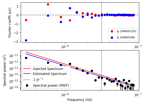
Estimating the spectral parameters from the DMWaveX fit.
[16]:
# Get the Fourier amplitudes and powers and their uncertainties.
# Note that the `DMWaveX` amplitudes have the units of DM.
# We multiply them by a constant factor to convert them to dimensions
# of time so that they are consistent with `PLDMNoise`.
scale = DMconst / (1400 * u.MHz) ** 2

idxs = np.array(m2.components["DMWaveX"].get_indices())
a = np.array(
    [(scale * m2[f"DMWXSIN_{idx:04d}"].quantity).to_value("s") for idx in idxs]
)
da = np.array(
    [(scale * m2[f"DMWXSIN_{idx:04d}"].uncertainty).to_value("s") for idx in idxs]
)
b = np.array(
    [(scale * m2[f"DMWXCOS_{idx:04d}"].quantity).to_value("s") for idx in idxs]
)
db = np.array(
    [(scale * m2[f"DMWXCOS_{idx:04d}"].uncertainty).to_value("s") for idx in idxs]
)
print(len(idxs))

P = (a**2 + b**2) / 2
dP = ((a * da) ** 2 + (b * db) ** 2) ** 0.5

f0 = (1 / Tspan).to_value(u.Hz)
fyr = (1 / u.year).to_value(u.Hz)
30
[17]:
# We can create a `PLDMNoise` model from the `DMWaveX` model.
# This will estimate the spectral parameters from the `DMWaveX`
# amplitudes.
m3 = pldmnoise_from_dmwavex(m2)
print(m3)
# Created: 2026-05-01T15:05:12.081368
# PINT_version: 1.1.4+112.g3f5c736
# User: docs
# Host: build-32499821-project-85767-nanograv-pint
# OS: Linux-7.0.0-1004-aws-x86_64-with-glibc2.35
# Python: 3.11.14 (main, Apr 27 2026, 17:28:30) [GCC 11.4.0]
# Format: pint
# read_time: 2026-05-01T15:04:16.567219
# allow_tcb: False
# convert_tcb: False
# allow_T2: False
PSR                                  SIM4
EPHEM                               DE440
CLOCK                        TT(BIPM2019)
UNITS                                 TDB
START              53000.9999999567105903
FINISH             56985.0000000465773148
DILATEFREQ                              N
DMDATA                                  N
NTOA                                 2000
CHI2                   1898.4189306027733
CHI2R                  0.9821101555110053
TRES               0.97321526471865212683
RAJ                      4:59:59.99999934 1 0.00000185847524176867
DECJ                    14:59:59.99976765 1 0.00016145911506297193
PMRA                                  0.0
PMDEC                                 0.0
PX                                    0.0
F0                  99.999999999999960205 1 3.5775429124952155762e-14
F1              -1.0000005446635623846e-15 1 8.169821965702234221e-22
PEPOCH             55000.0000000000000000
PLANET_SHAPIRO                          N
DM                  15.000007761618252591 1 4.967224699950917705e-06
TNDMAMP               -13.102122173341625 0 0.04398770724512381
TNDMGAM                3.4181016532188844 0 0.26424729237921035
TNDMC                                  30
TZRMJD             55000.0000000000000000
TZRSITE                               gbt
TZRFRQ                             1400.0
PHOFF               5.584696659776278e-05 1 5.504559749676612e-06
[18]:
# Now let us plot the estimated spectrum with the injected
# spectrum.
plt.subplot(211)
plt.errorbar(
    idxs * f0,
    b * 1e6,
    db * 1e6,
    ls="",
    marker="o",
    label="$\\hat{a}_j$ (DMWXCOS)",
    color="red",
)
plt.errorbar(
    idxs * f0,
    a * 1e6,
    da * 1e6,
    ls="",
    marker="o",
    label="$\\hat{b}_j$ (DMWXSIN)",
    color="blue",
)
plt.axvline(fyr, color="black", ls="dotted")
plt.axhline(0, color="grey", ls="--")
plt.ylabel("Fourier coeffs ($\mu$s)")
plt.xscale("log")
plt.legend(fontsize=8)

plt.subplot(212)
plt.errorbar(
    idxs * f0, P, dP, ls="", marker="o", label="Spectral power (PINT)", color="k"
)
P_inj = m.components["PLDMNoise"].get_noise_weights(t)[::2][:nharm_opt]
plt.plot(idxs * f0, P_inj, label="Injected Spectrum", color="r")
P_est = m3.components["PLDMNoise"].get_noise_weights(t)[::2][:nharm_opt]
print(len(idxs), len(P_est))
plt.plot(idxs * f0, P_est, label="Estimated Spectrum", color="b")
plt.xscale("log")
plt.yscale("log")
plt.ylabel("Spectral power (s$^2$)")
plt.xlabel("Frequency (Hz)")
plt.axvline(fyr, color="black", ls="dotted", label="1 yr$^{-1}$")
plt.legend()
30 30
[18]:
<matplotlib.legend.Legend at 0x7854ec7e8f90>
Chromatic noise fitting
Let us now do a similar kind of analysis for chromatic noise.
[19]:
par_sim = """
    PSR           SIM5
    RAJ           05:00:00     1
    DECJ          15:00:00     1
    PEPOCH        55000
    F0            100          1
    F1            -1e-15       1
    PHOFF         0            1
    DM            15
    CM            1.2          1
    TNCHROMIDX    3.5
    TNCHROMAMP    -13
    TNCHROMGAM    3.5
    TNCHROMC      30
    TZRMJD        55000
    TZRFRQ        1400
    TZRSITE       gbt
    UNITS         TDB
    EPHEM         DE440
    CLOCK         TT(BIPM2019)
"""

m = get_model(StringIO(par_sim))
[20]:
# Generate the simulated TOAs.
ntoas = 2000
toaerrs = np.random.uniform(0.5, 2.0, ntoas) * u.us
freqs = np.linspace(500, 1500, 8) * u.MHz

t = make_fake_toas_uniform(
    startMJD=53001,
    endMJD=57001,
    ntoas=ntoas,
    model=m,
    freq=freqs,
    obs="gbt",
    error=toaerrs,
    add_noise=True,
    add_correlated_noise=True,
    name="fake",
    include_bipm=True,
    multi_freqs_in_epoch=True,
)
[21]:
# Find the optimum number of harmonics by minimizing AIC.
m1 = deepcopy(m)
m1.remove_component("PLChromNoise")

m2 = deepcopy(m1)

nharm_opt = m.TNCHROMC.value
[22]:
# Now create a new model with the optimum number of
# harmonics
m2 = deepcopy(m1)

Tspan = t.get_mjds().max() - t.get_mjds().min()
cmwavex_setup(m2, T_span=Tspan, n_freqs=nharm_opt, freeze_params=False)

ftr = WLSFitter(t, m2)
ftr.fit_toas(maxiter=10)
m2 = ftr.model

print(m2)
# Created: 2026-05-01T15:05:21.586738
# PINT_version: 1.1.4+112.g3f5c736
# User: docs
# Host: build-32499821-project-85767-nanograv-pint
# OS: Linux-7.0.0-1004-aws-x86_64-with-glibc2.35
# Python: 3.11.14 (main, Apr 27 2026, 17:28:30) [GCC 11.4.0]
# Format: pint
# read_time: 2026-05-01T15:05:12.665673
# allow_tcb: False
# convert_tcb: False
# allow_T2: False
PSR                                  SIM5
EPHEM                               DE440
CLOCK                        TT(BIPM2019)
UNITS                                 TDB
START              53000.9999999566952084
FINISH             56985.0000000450458796
DILATEFREQ                              N
DMDATA                                  N
NTOA                                 2000
CHI2                   1863.5847444523588
CHI2R                  0.9640893659867351
TRES               0.97664319864910921796
RAJ                      5:00:00.00000129 1 0.00000146110423846528
DECJ                    15:00:00.00006585 1 0.00012585082999786153
PMRA                                  0.0
PMDEC                                 0.0
PX                                    0.0
F0                 100.000000000000029074 1 2.8838798476727667927e-14
F1              -9.9999792433562539195e-16 1 6.4987811159978614485e-22
PEPOCH             55000.0000000000000000
PLANET_SHAPIRO                          N
DM                                   15.0
CM                  1.1837103591258850697 1 0.05195413807825014635
TNCHROMIDX                            3.5
CMWXEPOCH          55000.0000000000000000
CMWXFREQ_0001       0.0002510040160586906
CMWXSIN_0001           153.43669456899346 1 0.0676360480223919
CMWXCOS_0001            91.40583927366532 1 0.07286716448769852
CMWXFREQ_0002       0.0005020080321173812
CMWXSIN_0002            70.63975468488539 1 0.06256616708381811
CMWXCOS_0002            16.88694255150641 1 0.05832498079595632
CMWXFREQ_0003       0.0007530120481760718
CMWXSIN_0003           -3.166001385255612 1 0.05964514996991725
CMWXCOS_0003             9.32172242113326 1 0.05920961686176122
CMWXFREQ_0004       0.0010040160642347624
CMWXSIN_0004          -14.961394378896227 1 0.0595943423911195
CMWXCOS_0004            4.017294365364037 1 0.05844142316551658
CMWXFREQ_0005        0.001255020080293453
CMWXSIN_0005           -4.475224780473841 1 0.058368476057081
CMWXCOS_0005            3.644244355396789 1 0.059266648984472634
CMWXFREQ_0006       0.0015060240963521436
CMWXSIN_0006           -8.799198121825043 1 0.059912467696452136
CMWXCOS_0006           -9.247443152960718 1 0.05759783392747788
CMWXFREQ_0007       0.0017570281124108342
CMWXSIN_0007             5.24122039618062 1 0.05843712956799607
CMWXCOS_0007         -0.24904323804261397 1 0.059018263004775244
CMWXFREQ_0008        0.002008032128469525
CMWXSIN_0008          0.38966360799147737 1 0.05754017237575536
CMWXCOS_0008           5.4735903496836595 1 0.05975249877057516
CMWXFREQ_0009        0.002259036144528215
CMWXSIN_0009           3.9489266136104115 1 0.05844145558849171
CMWXCOS_0009          -0.9908884660121895 1 0.058890428199618726
CMWXFREQ_0010        0.002510040160586906
CMWXSIN_0010          -3.1766566060184593 1 0.058056233910316626
CMWXCOS_0010          -0.8096052569781303 1 0.05949960753701936
CMWXFREQ_0011       0.0027610441766455964
CMWXSIN_0011         -0.23898111534944802 1 0.07379619334817851
CMWXCOS_0011          -3.0488493465980793 1 0.07216591922848356
CMWXFREQ_0012       0.0030120481927042872
CMWXSIN_0012           -1.413894580471874 1 0.057589958826255054
CMWXCOS_0012          -1.4833367545789518 1 0.05974906168280258
CMWXFREQ_0013       0.0032630522087629776
CMWXSIN_0013           0.8945569349409492 1 0.058539033603807876
CMWXCOS_0013         -0.07170628943117198 1 0.05889617575392724
CMWXFREQ_0014       0.0035140562248216684
CMWXSIN_0014           3.1406286387758686 1 0.0600412604997121
CMWXCOS_0014           2.0698937243940816 1 0.05734575326333838
CMWXFREQ_0015        0.003765060240880359
CMWXSIN_0015         -0.49339034424450634 1 0.058686471278573495
CMWXCOS_0015         -0.04347604343460379 1 0.05860042177539298
CMWXFREQ_0016         0.00401606425693905
CMWXSIN_0016           1.6803541719368948 1 0.05830422419724511
CMWXCOS_0016          -0.4630417654257609 1 0.05904877894265835
CMWXFREQ_0017         0.00426706827299774
CMWXSIN_0017           1.2551052268446732 1 0.05741984889640276
CMWXCOS_0017         -0.33705168445383554 1 0.059994265604586684
CMWXFREQ_0018         0.00451807228905643
CMWXSIN_0018           0.9065833375632577 1 0.058330947283956776
CMWXCOS_0018           1.4422784121953933 1 0.05879807696975964
CMWXFREQ_0019        0.004769076305115121
CMWXSIN_0019           1.5904931241301805 1 0.05705235836074917
CMWXCOS_0019          -0.6163850115199473 1 0.060009346951398146
CMWXFREQ_0020        0.005020080321173812
CMWXSIN_0020          0.16361301064102948 1 0.058668523601106776
CMWXCOS_0020          -1.7029655809100637 1 0.058560112772814754
CMWXFREQ_0021        0.005271084337232502
CMWXSIN_0021           0.6258099045235539 1 0.05890532391388282
CMWXCOS_0021           1.0904161229855198 1 0.05839527307039406
CMWXFREQ_0022        0.005522088353291193
CMWXSIN_0022         0.029621642591253248 1 0.060292091689947855
CMWXCOS_0022         0.043705582515902716 1 0.05696395406702115
CMWXFREQ_0023        0.005773092369349884
CMWXSIN_0023           0.5824996256222813 1 0.059398478951491064
CMWXCOS_0023          0.13298888937567152 1 0.057932526267608246
CMWXFREQ_0024       0.0060240963854085745
CMWXSIN_0024           0.5507974095913124 1 0.058587030470462494
CMWXCOS_0024        0.0008942782909823268 1 0.058557948710029166
CMWXFREQ_0025        0.006275100401467264
CMWXSIN_0025           -0.313919308998523 1 0.060261798050615996
CMWXCOS_0025          -0.5188024246917678 1 0.056918324343090326
CMWXFREQ_0026        0.006526104417525955
CMWXSIN_0026         -0.20316496494051894 1 0.05823337529303369
CMWXCOS_0026         -0.17528048315030595 1 0.05895355529351421
CMWXFREQ_0027        0.006777108433584646
CMWXSIN_0027          0.14690937678276794 1 0.05889297142050177
CMWXCOS_0027           0.3916730452849484 1 0.058260006893542826
CMWXFREQ_0028        0.007028112449643337
CMWXSIN_0028         -0.35252682018494763 1 0.05898752452553252
CMWXCOS_0028         -0.07563136610709283 1 0.0582391357124357
CMWXFREQ_0029        0.007279116465702027
CMWXSIN_0029          0.08916230186844512 1 0.05841443778126037
CMWXCOS_0029          0.41993451945916477 1 0.05879668858510578
CMWXFREQ_0030        0.007530120481760718
CMWXSIN_0030          -0.3092616094821627 1 0.059111156385783174
CMWXCOS_0030          0.04102661959091234 1 0.057880220548265464
TZRMJD             55000.0000000000000000
TZRSITE                               gbt
TZRFRQ                             1400.0
PHOFF               0.0004833675267758922 1 4.256144332178786e-06
Estimating the spectral parameters from the CMWaveX fit.
[23]:
# Get the Fourier amplitudes and powers and their uncertainties.
# Note that the `CMWaveX` amplitudes have the units of pc/cm^3/MHz^2.
# We multiply them by a constant factor to convert them to dimensions
# of time so that they are consistent with `PLChromNoise`.
scale = DMconst / 1400**m.TNCHROMIDX.value

idxs = np.array(m2.components["CMWaveX"].get_indices())
a = np.array(
    [(scale * m2[f"CMWXSIN_{idx:04d}"].quantity).to_value("s") for idx in idxs]
)
da = np.array(
    [(scale * m2[f"CMWXSIN_{idx:04d}"].uncertainty).to_value("s") for idx in idxs]
)
b = np.array(
    [(scale * m2[f"CMWXCOS_{idx:04d}"].quantity).to_value("s") for idx in idxs]
)
db = np.array(
    [(scale * m2[f"CMWXCOS_{idx:04d}"].uncertainty).to_value("s") for idx in idxs]
)
print(len(idxs))

P = (a**2 + b**2) / 2
dP = ((a * da) ** 2 + (b * db) ** 2) ** 0.5

f0 = (1 / Tspan).to_value(u.Hz)
fyr = (1 / u.year).to_value(u.Hz)
30
[24]:
# We can create a `PLChromNoise` model from the `CMWaveX` model.
# This will estimate the spectral parameters from the `CMWaveX`
# amplitudes.
m3 = plchromnoise_from_cmwavex(m2)
print(m3)
# Created: 2026-05-01T15:05:21.644757
# PINT_version: 1.1.4+112.g3f5c736
# User: docs
# Host: build-32499821-project-85767-nanograv-pint
# OS: Linux-7.0.0-1004-aws-x86_64-with-glibc2.35
# Python: 3.11.14 (main, Apr 27 2026, 17:28:30) [GCC 11.4.0]
# Format: pint
# read_time: 2026-05-01T15:05:12.665673
# allow_tcb: False
# convert_tcb: False
# allow_T2: False
PSR                                  SIM5
EPHEM                               DE440
CLOCK                        TT(BIPM2019)
UNITS                                 TDB
START              53000.9999999566952084
FINISH             56985.0000000450458796
DILATEFREQ                              N
DMDATA                                  N
NTOA                                 2000
CHI2                   1863.5847444523588
CHI2R                  0.9640893659867351
TRES               0.97664319864910921796
RAJ                      5:00:00.00000129 1 0.00000146110423846528
DECJ                    15:00:00.00006585 1 0.00012585082999786153
PMRA                                  0.0
PMDEC                                 0.0
PX                                    0.0
F0                 100.000000000000029074 1 2.8838798476727667927e-14
F1              -9.9999792433562539195e-16 1 6.4987811159978614485e-22
PEPOCH             55000.0000000000000000
PLANET_SHAPIRO                          N
DM                                   15.0
CM                  1.1837103591258850697 1 0.05195413807825014635
TNCHROMIDX                            3.5
TZRMJD             55000.0000000000000000
TZRSITE                               gbt
TZRFRQ                             1400.0
PHOFF               0.0004833675267758922 1 4.256144332178786e-06
TNCHROMAMP            -13.012516771038264 0 0.0401344462583141
TNCHROMGAM              3.537761089242865 0 0.24207920594428206
TNCHROMC                               30
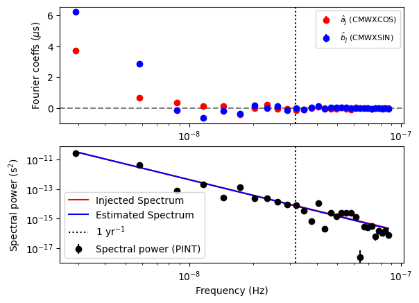
[25]:
# Now let us plot the estimated spectrum with the injected
# spectrum.
plt.subplot(211)
plt.errorbar(
    idxs * f0,
    b * 1e6,
    db * 1e6,
    ls="",
    marker="o",
    label="$\\hat{a}_j$ (CMWXCOS)",
    color="red",
)
plt.errorbar(
    idxs * f0,
    a * 1e6,
    da * 1e6,
    ls="",
    marker="o",
    label="$\\hat{b}_j$ (CMWXSIN)",
    color="blue",
)
plt.axvline(fyr, color="black", ls="dotted")
plt.axhline(0, color="grey", ls="--")
plt.ylabel("Fourier coeffs ($\mu$s)")
plt.xscale("log")
plt.legend(fontsize=8)

plt.subplot(212)
plt.errorbar(
    idxs * f0, P, dP, ls="", marker="o", label="Spectral power (PINT)", color="k"
)
P_inj = m.components["PLChromNoise"].get_noise_weights(t)[::2]
plt.plot(idxs * f0, P_inj, label="Injected Spectrum", color="r")
P_est = m3.components["PLChromNoise"].get_noise_weights(t)[::2]
print(len(idxs), len(P_est))
plt.plot(idxs * f0, P_est, label="Estimated Spectrum", color="b")
plt.xscale("log")
plt.yscale("log")
plt.ylabel("Spectral power (s$^2$)")
plt.xlabel("Frequency (Hz)")
plt.axvline(fyr, color="black", ls="dotted", label="1 yr$^{-1}$")
plt.legend()
30 30
[25]:
<matplotlib.legend.Legend at 0x7854dfda13d0>
[ ]: